
Introduction
In my long-term trading strategy, I focus on determining the intrinsic value of a stock by examining the company’s core financials and adjusting the valuation through market risk factors. I employ the discounted cash flow (DCF) model to estimate a company’s enterprise and equity values based on future cash flows. Moreover, to capture systematic market risk, I incorporate elements from the French Fama 3 Factor model by integrating risk‐free rate data from Ken French’s dataset into my cost of equity calculations. This dual approach merges internal growth dynamics with external market behavior.
Data Sources and Key Variables
To perform the analysis, I extract several data points from the company’s financial statements:
- Enterprise Value (EV): Fetched using API endpoints from a financial data provider.
- Income Statement Items: Operating Income, Income Before Tax, Income Tax Expense, and Interest Expense.
- Balance Sheet Components: Market Capitalization, Total Assets, Total Non-Current Assets, Debt, and Cash Equivalents.
- Cash Flow Statement Components: Capital Expenditure and Depreciation & Amortization.
From these, I compute key variables such as the Discount Rate (WACC), Earnings and CapEx Growth Rates (using the compound annual growth rate), and the Perpetual Growth Rate—often proxied by the risk‐free rate.
Methodological Framework
Discounted Cash Flow (DCF) Model
The DCF model is central to my valuation process. By projecting future unlevered free cash flows (ULFCF) over a forecast period, discounting them at the appropriate WACC, and adding a terminal value, I calculate the enterprise value of a company. Below is a code snippet from my data-dcf.py file that demonstrates the computation of the enterprise value.
def enterprise_value(income_statement, cashflow_statement, balance_statement, period, discount_rate, earnings_growth_rate, cap_ex_growth_rate, perpetual_growth_rate):
if income_statement[0]['operatingIncome']:
ebit = float(income_statement[0]['operatingIncome'])
else:
earnings_before_tax = float(income_statement[0]['incomeBeforeTax'])
interest_expense = float(income_statement[0]['interestExpense'])
ebit = earnings_before_tax - interest_expense
tax_rate = float(income_statement[0]['incomeTaxExpense']) / float(income_statement[0]['incomeBeforeTax'])
non_cash_charges = float(cashflow_statement[1]['depreciationAndAmortization'])
cwc = (float(balance_statement[0]['totalAssets']) - float(balance_statement[0]['totalNonCurrentAssets'])) - \
(float(balance_statement[1]['totalAssets']) - float(balance_statement[1]['totalNonCurrentAssets']))
cap_ex = float(cashflow_statement[0]['capitalExpenditure'])
discount = discount_rate
flows = []
for yr in range(1, period+1):
ebit = ebit * (1 + earnings_growth_rate)**yr
non_cash_charges = non_cash_charges * (1 + (yr * earnings_growth_rate))
cwc = cwc * 0.7
cap_ex = cap_ex * (1 + cap_ex_growth_rate)**yr
flow = ulFCF(ebit, tax_rate, non_cash_charges, cwc, cap_ex)
PV_flow = flow/((1 + discount)**yr)
flows.append(PV_flow)
NPV_FCF = sum(flows)
final_cashflow = flows[-1] * (1 + perpetual_growth_rate)
TV = final_cashflow/(discount - perpetual_growth_rate)
NPV_TV = TV/(1+discount)**(1+period)
return NPV_TV + NPV_FCF
Incorporating the French Fama Model
To estimate the cost of equity, I implement a regression framework derived from the French Fama 3 Factor model. By extracting the risk-free rate from Ken French’s dataset and adjusting market returns, I perform an OLS regression to estimate the stock’s beta and alpha. The cost of equity is then calculated as:
Cost of Equity = Risk Free Rate + β × (Annualized Market Return - Risk Free Rate)
The following code snippet (again from data-dcf_py.py) illustrates this process. :contentReference[oaicite:1]{index=1}
def get_cost_of_equity():
end_str = '2024-01-02' # Consider current date
end = pd.to_datetime(end_str).date()
start = end - pd.DateOffset(years=1)
input_symbols = ['^GSPC','SMCI']
adj_closes = {}
for symbol in input_symbols:
data = yf.download(symbol, start=start, end=end)
adj_closes[symbol] = data['Adj Close']
df = pd.DataFrame(adj_closes)
df_returns = df.pct_change()
df_returns_m = df_returns.resample('M').agg(lambda x: (x+1).prod()-1)[1:-1]
df_returns_m.index = df_returns_m.index.to_period('M')
ff_factors = reader.DataReader('F-F_Research_Data_5_Factors_2x3','famafrench', start, end)[0].RF[1:]
df_returns_m['^GSPC-rf'] = df_returns_m['^GSPC'] - ff_factors
df_returns_m['SMCI-rf'] = df_returns_m['SMCI'] - ff_factors
y = df_returns_m['SMCI-rf']
X = df_returns_m['^GSPC-rf']
X_sm = sm.add_constant(X)
results = sm.OLS(y, X_sm).fit()
stock_beta = results.params['^GSPC-rf']
risk_free_rate = ff_factors.mean()
average_market_return = df_returns_m['^GSPC'].mean()
df_returns_annual = (1 + average_market_return)**12 - 1
cost_of_equity = risk_free_rate + stock_beta * (df_returns_annual - risk_free_rate)
return cost_of_equity
Weighted Average Cost of Capital (WACC)
The cost of equity, in combination with the cost of debt, is blended to derive the WACC, which is used as the discount rate in the DCF calculation. The snippet below shows how I compute the WACC:
def get_discount_rate(income_statement):
tax_rate = float(income_statement[0]['incomeTaxExpense']) / float(income_statement[0]['incomeBeforeTax'])
cost_of_debt = income_statement[0]['interestExpense'] / ev_statement[0]['addTotalDebt']
weight_of_equity = ev_statement[0]['marketCapitalization'] / (ev_statement[0]['marketCapitalization'] + ev_statement[0]['addTotalDebt'])
weight_of_debt = ev_statement[0]['addTotalDebt'] / (ev_statement[0]['marketCapitalization'] + ev_statement[0]['addTotalDebt'])
wacc = (weight_of_equity * get_cost_of_equity()) + (weight_of_debt * cost_of_debt * (1 - tax_rate))
return wacc
System Architecture and Implementation
My project is modularized across several Python files:
- data-dcf_py.py: Contains core computations for DCF valuation, discount rate derivation, and growth rate calculations.
- main.py: Serves as the entry point, parsing command-line arguments and orchestrating data fetching and analysis. (:contentReference[oaicite:3]{index=3})
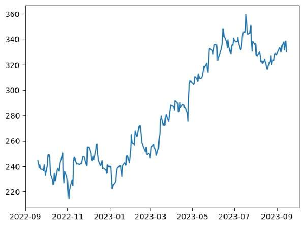
- plot_calc.py: Includes functions to create visual representations such as trend graphs and rolling averages. (:contentReference[oaicite:4]{index=4})
- ticker_module.py: Provides helper methods for ticker validation and data retrieval from Yahoo Finance. (:contentReference[oaicite:5]{index=5})
The following excerpt from main.py demonstrates how I fetch data and execute the analysis:
def main():
parser = argparse.ArgumentParser(description='Perform analysis on stock data')
parser.add_argument('ticker_list', nargs='+', help='List of tickers. The first ticker should start with "^".')
parser.add_argument('--start_date', type=str, help='Start date for fetching data (YYYY-MM-DD format)')
parser.add_argument('--period_type', choices=['daily', 'weekly', 'monthly', 'yearly'], help='Type of period for fetching data')
parser.add_argument('--num_periods', type=int, help='Number of periods for fetching data')
args = parser.parse_args()
tickers = ticker_list(args.ticker_list)
start_date, df = fetch_data_for_period(start_date=args.start_date, period_type=args.period_type, num_periods=args.num_periods, ticker_list=tickers)
plot_based_calculation(args.ticker_list, df, pd.to_datetime(start_date))
Next Steps: Annual Intrinsic Price Evaluation and Trend Analysis
The current implementation calculates the intrinsic stock price based on a snapshot of recent annual financial data. The next steps in the process include:
- Yearly Valuation: Iterate through historical financial data to compute the intrinsic price for each year using the DCF model.
- Deviation Analysis: Compare the calculated intrinsic values with actual market prices to measure the percentage difference and margin of safety.
- Trend Plotting: Use graphical analysis (via functions in plot_calc.py) to visualize trends over time, including trend lines and rolling averages that capture how market valuations deviate from intrinsic estimates.
This extended analysis will offer insights into the reliability of the intrinsic valuation method over multiple years and support more informed long-term trading decisions.
Conclusion
By integrating in-depth company financials with an advanced market risk model based on the French Fama 3 Factor framework, I have developed a robust methodology for intrinsic stock valuation. The incorporation of risk‐free rate data and regression-based cost of equity calculations refines the discount rate within the DCF model. Moving forward, an annual evaluation paired with trend analysis will provide essential insights into the evolving relationship between market prices and intrinsic values, ultimately enhancing long-term investment strategies.
This research underscores the importance of a multi-dimensional approach to valuation—one that seamlessly blends fundamental analysis with real-world market dynamics.