

1. Introduction
This study examines Starbucks sales data over time with the primary goal of understanding the trend behavior and identifying drivers behind sales dynamics. Data obtained from WRDS provides quarterly observations, which are utilized to estimate various regression models. Both level and log transformations of sales are considered alongside models that incorporate lagged differences to account for time-dependent effects. This multifaceted approach allows for a deeper insight into how sales evolve and what factors contribute to their variation.
2. Data and Methodology
Data Source and Variables
The analysis uses quarterly data for Starbucks sales with a total of 76 observations in the primary datasets. Key variables include:
- Sales: Actual sales figures.
- Log(Sales): Logarithmic transformation of sales to analyze growth in percentage terms.
- Time: A sequential variable representing the time period.
- Lagged and Differenced Variables:
- lag1: The sales value one quarter behind.
- Diff1: The change calculated as the first difference of lagged sales.
- lag4_diff: The four-quarter lag on the differenced variable, used as part of a multivariate regression model to assess seasonal or delayed effects.
- Lagged and Differenced Variables:
- X Variables: In the final multivariate model, two explanatory variables (denoted as X Variable 1 and X Variable 2) are introduced to capture additional dynamics in the lagged effects.
Methodological Approach
The study estimates four key models:
- Model 1 (Sales vs. Time) – A simple linear regression exploring how sales change over time.
- Model 2 (Log(Sales) vs. Time) – A regression where the natural logarithm of sales is modeled as a function of time, indicating the growth rate.
- Model 3 (Diff1 vs. Time) – A model incorporating the first differenced lag variable to capture short-run adjustments.
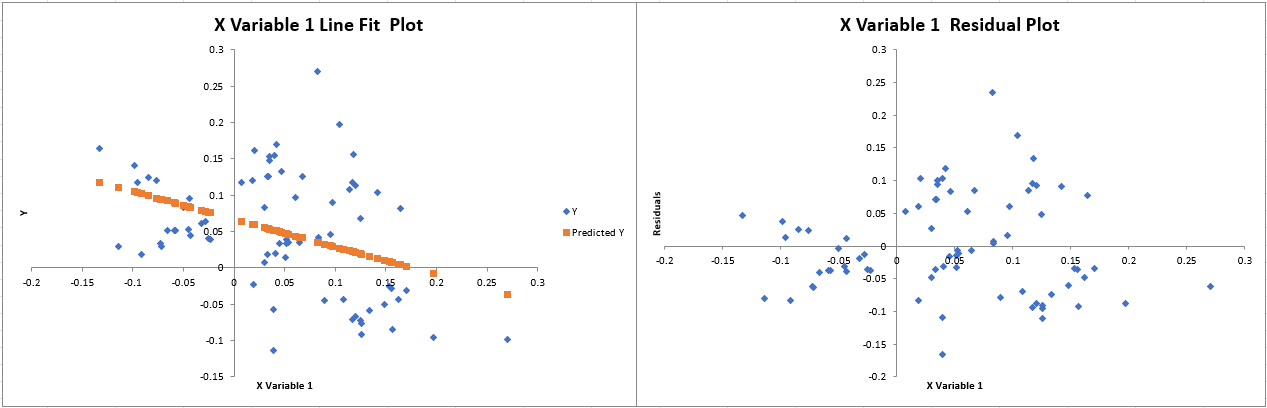
- Model 4 (Multivariate Regression with Lagged Differences) – A regression that uses a four-quarter lag differenced variable along with two predictors (X Variable 1 and X Variable 2) to better explain sales dynamics.
- Time Trend and Growth:
Both the level and log models (Models 1 and 2) indicate a strong upward trend in sales. The high R Square values (0.9595 and 0.9453) and significant time coefficients underscore that time is the primary driver of sales increase. - Log Transformation Insights:
Model 2’s log transformation provides a clear interpretation in terms of growth percentages. This is valuable for assessing relative changes over time. - Short-Run Dynamics:
Model 3, which examines the first difference (Diff1), suggests that deviations from the long-run trend trigger adjustments. Even though the model’s explanatory power is lower, the significant negative coefficient signals possible mean-reversion behavior in the short-term dynamics of sales. - Lagged Effects and Multivariate Analysis:
The multivariate model (Model 4) introduces lagged difference variables and distinguishes between two predictors. The high overall model fit (R Square = 0.8162) indicates that the inclusion of lagged factors is crucial for explaining sales variability. In particular, the highly significant positive coefficient on X Variable 2 points to its influential role, while the insignificance of X Variable 1 suggests that not every lagged factor may be relevant. - Diagnostic Plots:
The placeholders for the line fit and residual plots are intended to assess the goodness-of-fit and potential model violations. For example, the Time Line Fit Plot and Time Residual Plot will help examine any patterns or autocorrelation in the error terms, while the fit and residual plots for X Variable 1 and X Variable 2 will provide further insight into the multivariate regression’s reliability. - Insert and analyze the respective diagnostic plots ([Time Line Fit Plot], [Time Residual Plot], [X Variable 1 Residual Plot], [X Variable 1 Line Fit Plot], [X Variable 2 Residual Plot], and [X Variable 2 Line Fit Plot]).
- Validate model assumptions such as homoscedasticity and absence of autocorrelation.
- Consider incorporating additional explanatory variables to further refine the model.
For each model, both the regression statistics and the ANOVA results have been carefully examined.
3. Regression Results
Model 1: Sales as a Function of Time
| Multiple R | 0.979562298 |
|---|---|
| R Square | 0.959542295 |
| Adjusted R Square | 0.958995569 |
| Standard Error | 233.2115638 |
| Observations | 76 |
| df | SS | MS | F | Significance F | |
|---|---|---|---|---|---|
| Regression | 1 | 95454137.77 | 95454137.77 | 1755.070623 | 2.71413E-53 |
| Residual | 74 | 4024684.878 | 54387.63348 | ||
| Total | 75 | 99478822.65 |
| Coefficients | Standard Error | t Stat | P-value | Lower 95% | Upper 95% | |
|---|---|---|---|---|---|---|
| Intercept | -428.5281095 | 54.03477737 | -7.930598224 | 1.75211E-11 | -536.1947536 | -320.8614653 |
| time | 51.08638972 | 1.219432916 | 41.89356303 | 2.71413E-53 | 48.6566166 | 53.51616284 |
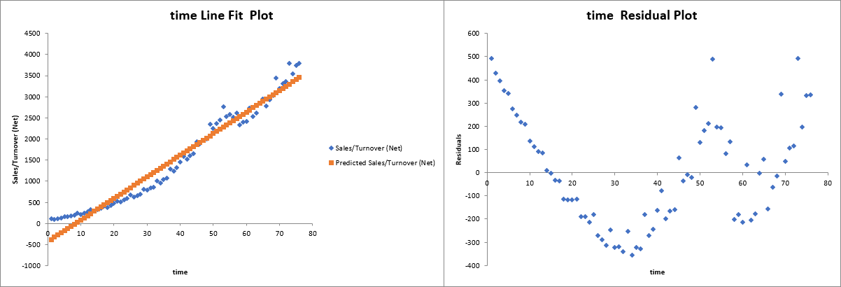
Interpretation: The high R square indicates that approximately 96% of the variability in sales is explained by the time trend. The positive coefficient on time suggests that Starbucks sales are increasing steadily over time.
Model 2: Log(Sales) as a Function of Time
| Multiple R | 0.972249052 |
|---|---|
| R Square | 0.94526822 |
| Adjusted R Square | 0.944528601 |
| Standard Error | 0.248189138 |
| Observations | 76 |
| df | SS | MS | F | Significance F | |
|---|---|---|---|---|---|
| Regression | 1 | 78.72501322 | 78.72501322 | 1278.048105 | 1.96161E-48 |
| Residual | 74 | 4.558240769 | 0.061597848 | ||
| Total | 75 | 83.28325399 |
| Coefficients | Standard Error | t Stat | P-value | Lower 95% | Upper 95% | |
|---|---|---|---|---|---|---|
| Intercept | 5.130345746 | 0.057505059 | 89.2155543 | 4.44712E-77 | 5.015764414 | 5.244927078 |
| time | 0.046394255 | 0.001297749 | 35.74979868 | 1.96161E-48 | 0.043808434 | 0.048980076 |
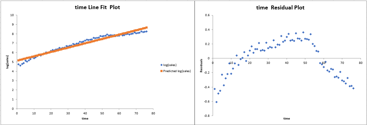
Interpretation: By transforming sales into its logarithm, the model captures percentage changes rather than absolute levels. The results imply a consistent growth rate over time, with time having a statistically significant positive effect on log(sales).
Model 3: First Differenced Regression (Diff1)
| Multiple R | 0.393399556 |
|---|---|
| R Square | 0.154763212 |
| Adjusted R Square | 0.143023812 |
| Standard Error | 0.076189131 |
| Observations | 74 |
| df | SS | MS | F | Significance F | |
|---|---|---|---|---|---|
| Regression | 1 | 0.076525799 | 0.076525799 | 13.18323033 | 0.000525376 |
| Residual | 72 | 0.41794442 | 0.005804784 | ||
| Total | 73 | 0.49447022 |
| Coefficients | Standard Error | t Stat | P-value | Lower 95% | Upper 95% | |
|---|---|---|---|---|---|---|
| Intercept | 0.066879078 | 0.010138108 | 6.596800656 | 6.06927E-09 | 0.046669128 | 0.087089025 |
| Diff1 | -0.381343864 | 0.105028181 | -3.630871842 | 0.000525376 | -0.590713716 | -0.171974012 |
Interpretation: This model, which focuses on the first difference of lagged sales, reveals a statistically significant negative relationship. Although the overall explanatory power is low (R Square ≈ 15%), the significant coefficient on Diff1 suggests short-term corrections or adjustments in sales levels.
Model 4: Multivariate Regression with Lagged Differences
| Multiple R | 0.903462253 |
|---|---|
| R Square | 0.816244042 |
| Adjusted R Square | 0.810839455 |
| Standard Error | 0.034053583 |
| Observations | 71 |
| df | SS | MS | F | Significance F | |
|---|---|---|---|---|---|
| Regression | 2 | 0.350278222 | 0.175139111 | 151.0280144 | 9.64292E-26 |
| Residual | 68 | 0.078855963 | 0.001159647 | ||
| Total | 70 | 0.429134185 |
| Coefficients | Standard Error | t Stat | P-value | Lower 95% | Upper 95% | |
|---|---|---|---|---|---|---|
| Intercept | 0.008398948 | 0.005852967 | 1.434989891 | 0.155873564 | -0.003280465 | 0.020078361 |
| X Variable 1 | -0.060218919 | 0.053957254 | -1.116048622 | 0.268329667 | -0.167888943 | 0.047451105 |
| X Variable 2 | 0.804704249 | 0.052375719 | 15.3640706 | 8.36055E-24 | 0.700190128 | 0.909218369 |
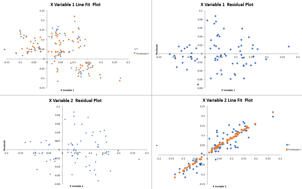
Interpretation: The multivariate model explains about 82% of the variability in sales differences, indicating a strong model fit. While X Variable 1 does not have a statistically significant impact, X Variable 2 is highly significant. This suggests that the second predictor—possibly representing a key lagged or seasonal factor—plays an important role in explaining changes in sales.
4. Discussion
The sequential modeling approach highlights several important aspects of the Starbucks sales data:
5. Conclusion
The regression analyses conducted on the Starbucks sales data reveal a robust and statistically significant time trend in both the level and log-transformed models. The short-run correction model (Model 3) and the multivariate lagged model (Model 4) further enhance the understanding of the dynamics at play. Notably, the strong influence of X Variable 2 in Model 4 suggests that some lagged factors have a critical impact on sales behavior. Future work may include a deeper exploration of autocorrelation issues and the potential for seasonal adjustments, which could offer additional insights into the persistence of sales trends.
Next Steps:
This case study provides a solid foundation for understanding Starbucks’ sales evolution through robust statistical modeling and paves the way for further analysis and forecasting.